NORA Documentation
- Introduction
- Viewer
- First Steps
- ROI-Tool
- Fiber Viewer
- Projects and Subject/Studies
- Autoloaders
- Marker-Tool
- Navigation Tool (alignment and deformations)
- URL Calls and Sharedlinks
- Reading Tool
- Data import
- Processing
- General
- Batchtool
- Jobs
- Jupyter Notebooks
- Fibertracking, Streamline Analysis
- Segmentation (Deep Learning)
- Installation
Introduction
What is NORA?
Nora is a general purpose medical imaging platform, which tries to fuse all aspects involved in modern clinical and fundamental imaging research.
It covers the following aspects
- Viewing:
a fully featured medical imaging viewer (like 3D slicer, ITK snap, etc.) and support of format slike DICOM, NIFTI, NRRD, MGH, GIFTI, TCK, .... - Annotations and Readings:
allow for high-throughput geometric and textual labeling/annotation of large datasets - Subject management and image archive
similar to frameworks like XNAT, but based on research format NIFTI. Additional non-imaging information is held as JSONs. - Image Processing:
include your favourite MATLAB tools, PYTHON tools, tensorflow, etc .. and apply on groups of subjects/study on a high perf. computing cluster. - Integration into clinical routine and research:
DICOM send/retrieve to allow easy pull (batch-import) and push to clinical systems. Automatic routing of image processing/analysis pipelines
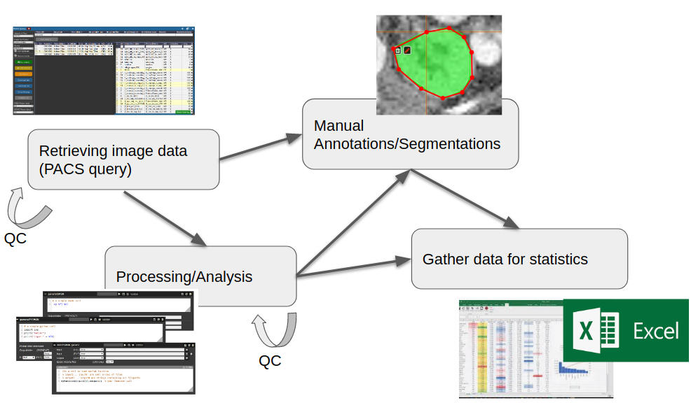
All these aspects are integrated into a multi-user web-frontend to organize collaborative research. A typical workflow starts with an image data query from your local PACS system. NORA provides to import imaging studies of large cohorts with a few clicks. The so called "autoloader" allows to easily browse the imported data in effective manner for quallity control (QC). The imported data can be preprocessed and analyzed by your favourite image processing tools (MATLAB, Python, BASH) and machine learning scripts. Annotation and labeling tools allow for an easy setup of segmentation/detection tasks with modern AI algorithms.
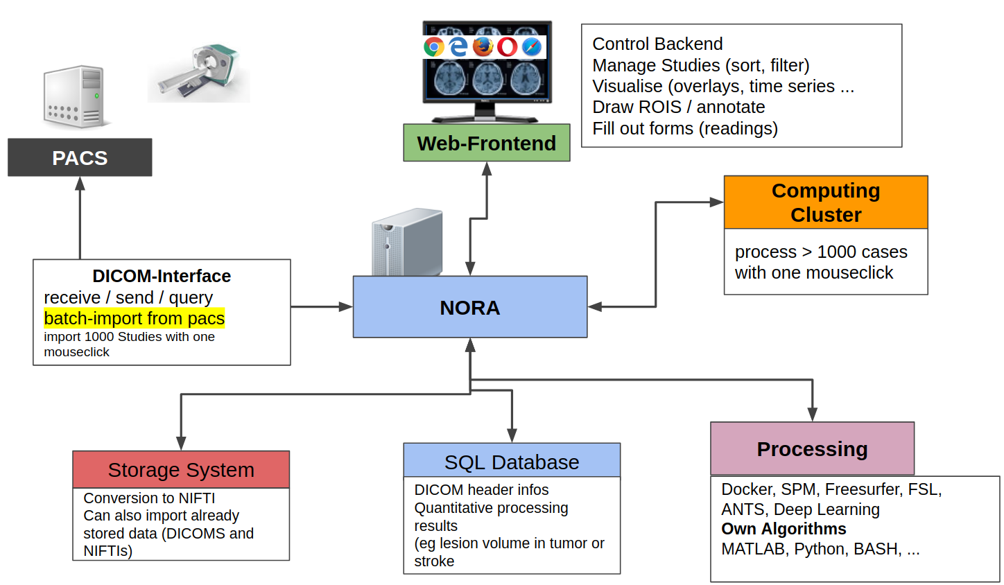
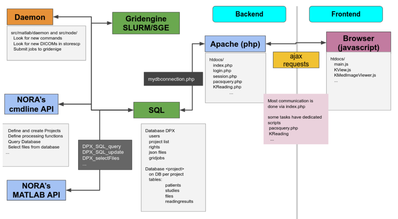
From the technical perspective NORA has a simple client/server architecture. Data is held on a central server/cloud storage and users have access to the system via a web-frontend. NORA's backend consists of a weberver (apache2, php7, nodejs), a computing cluster (Slurm or SGE/torque), DICOM nodes, and an SQL database (mysql). The SQL database holds
- Locations of imaging data items (basically NIFTI files, but also NRRD, MGH, GIFTI, TCK, TRK, STL, ...).
- Project information (collections of subjects/studies)
- User and access/rights information (synchronize with your LDAP/AD)
- Processing pipelines/scripts

Viewer
First Steps
Learning by doing is most of the times the best option. So, try out the demos on
to get an inital experience. Note that there is also a non-web version of the viewer (packed in electron) to allow local non-internet usage of the viewer (download also here)
NORA's desktop
NORA's basic working screen is like that: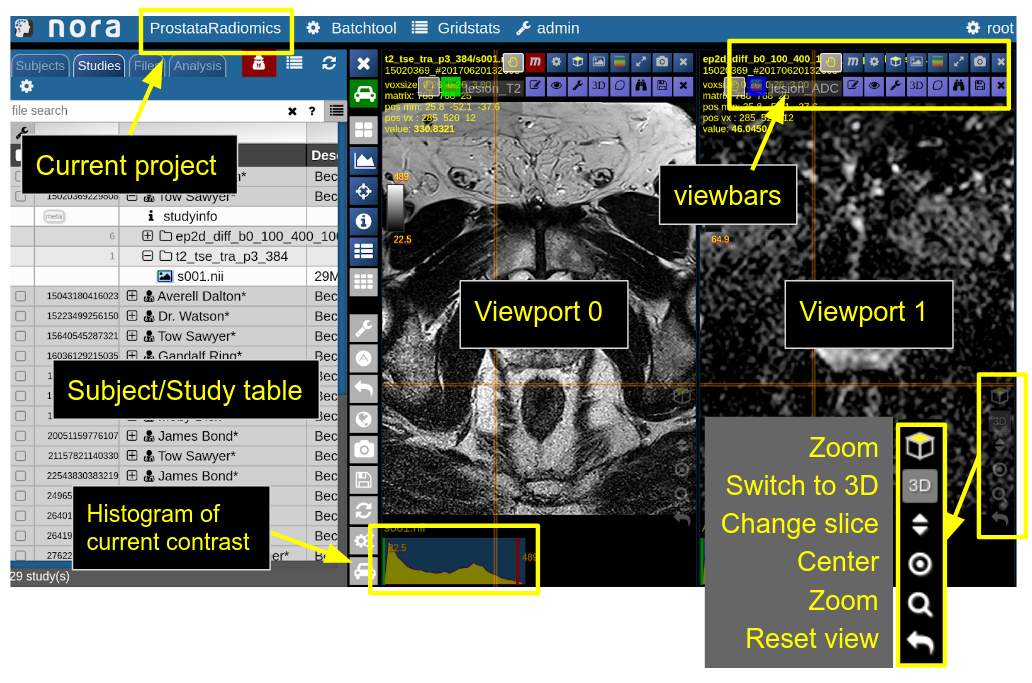
NORA's imaging data is organized in projects. Each projects contains a set of subjects/studies, which appear in the left table of the desktop.
Loading data for viewing happens in most of the cases per drag&drop. You can drag images from the subject/study table (see here for more about the table) into the viewports on the right. By double-clicking a file its content is loaded and placed into next available viewport. You can also drag&drop files from your local computer into the viewports for visulization (note that the data is not uploaded, it stays on your local machine).
Depending on the file type different drop options appear in the viewports. For example, if you want to overlay one image onto another just drop on "drop as overlay". Hence, each viewport can contain multiple items: a background, overlays, masks, fibers and surfaces (in 3D) etc.. Corresponding to each item a viewbar appears in the upper right corner of the viewport. The viewbar controls the appearence of the associated object/contrast. Most properties (colormapping, outlines, etc.) are set for all instances of the object in all viewports. If you want to choose the same object to have different appearence properties in different viewports use the shift key while selecting the property.
The viewbar of the "background" image is organzed as follows
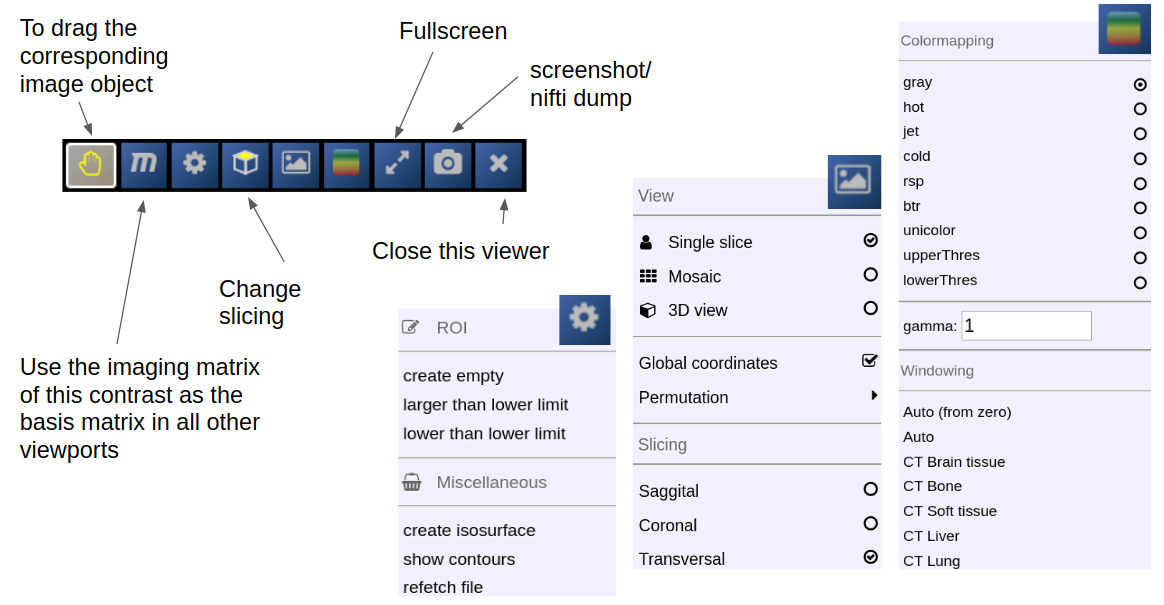
Central Toolbar
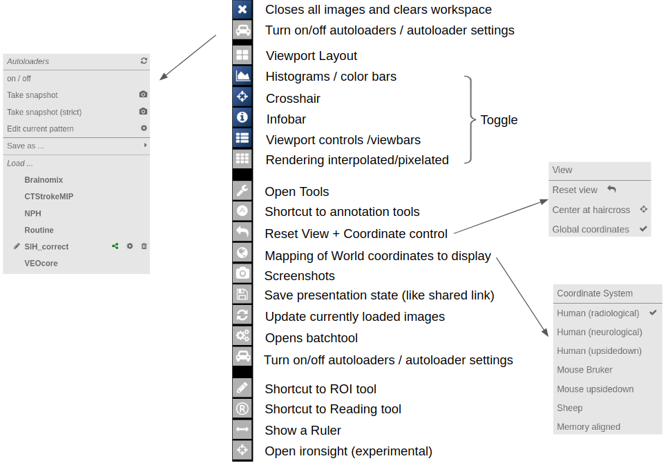
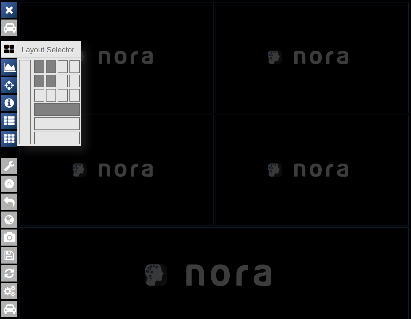
Viewports and Viewer Layout
To control the layout of the viewports use the layout selector located at the central toolbar. Note that for the horizontal viewports at the bottom a mosaic view is default.
Mouse
| Mouse wheel | change slice |
| Ctrl + Mouse wheel | zoom |
| Right mouse button (hold down) | pan |
| Left mouse buttom click | change position of crosshair (world position) |
| Middle mouse button | Change windowing |
| Ctrl + Left Mouse button hold | Reformatting MPR (rotation/translation) , see Navigation Tool |
Keyboard Shortcuts
| 1-6,0 | shortcuts to standard CT windowings |
| Space | toggle ROI edit, see ROI tool |
| s | open settings window |
| x,y | decrease/increase scroll speed |
| arrow up/down | change subject (when using autoloader) |
| (shift) Ctrl-Z | Undo/Redo ROI drawing |
ROI-Tool
 The ROI-Tool
The term Region of Interest (ROI) is used throughout the tutorial as a synonym for a "Mask", "Binary Mask", "Segmentation" or "Volume of Interest". Technically, it is a binary 3D volumetric image matrix, which is quite similar to 3D image apart from the fact that voxel values are binary (on or off). Thus, a ROI has also the same properties as image (like resolution and matrix size). ROIs can also be just 2D, however, one has to be remember that the 2D slice has also a position in 3D space, which can sometimes be confusing.
ROIs are close to what is represented by DICOM SEG objects.
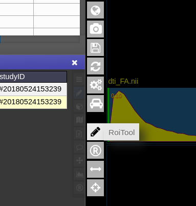
To open the ROI-tool just go via the toolbox menu of the vertical iconbar or use the shortcut via the "pen" icon:
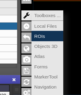
This opens the following toolbox window, which contains the access to all functionalities of the ROI-tool
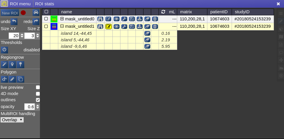
On the right you have list of currently opened ROIs togeter with information about matrix size and patientID/studyID. There is also information about the size of ROI and several tool icons:
|
focuses the position of the viewer to the center of gravity of the current ROI |
|
|
|
turns the ROI to be the "current ROI" on which currently is drawn on |
 |
toggles the visiblity of the ROI in all viewports |
 |
open several options to modfiy ROIs (see below: ROI operations) |
 |
save the ROI (upload to server) |
 |
downloads the ROI to your local computer |
 |
erases/clears all on voxels of the ROI |
 |
deletes the ROI from workspace |

Drawing and Pens
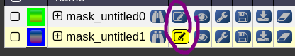
Generally, the left mouse button turns voxels on, while right mouse button eraśes voxels. Drawing happens always on the ROI which is currently selected for drawing. You can select
a ROI for drawing by highlighting the pencil icon in the viewbar, or in the ROItool
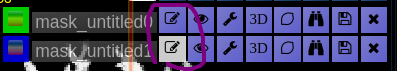
A shortcut for switching drawing on/off you cane use the spacebar. You can also hold shift pressed while being in drawing mode to disable mouse drawning features.
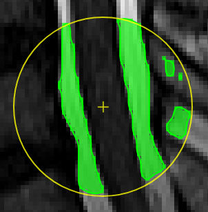
On the left panel of the ROI-tool the current type of pen mode (pen type) and the size of the pen can be set. You can turn on "live preview" to see what the current pen would draw. Displayed opacity of the ROI can be determined and whether outlines are drawn. The available pen types are as follows:
|
|
Thresholding based pen.Depending on the threshold (either choose clImL/R or an actual number) the pen turns voxels ON, which are above ("Higher") or below ("Lower") the threshold. Additional you can select "Higher RGrow"/"Lower RGrow" to enforce the ON voxels to be connected to the central voxel.
|
|
|
Magic pen (unconnected).Turns voxel ON, which have a 1) similar contrast compared to the central voxel, 2) are within pen's radius. The similarity depends on the color limits chosen for the current contrasts.
|
|
|
Magic pen (connected).Turns voxel ON, which have a 1) similar contrast compared to the central voxel, 2) are within pen's radius. and 3) are connected to central voxel via a region growing approach. The similarity depends on the color limits chosen for the current contrasts.
|
|
|
Unconstrained 3D region Growing.Select a pixel by keeping left mouse button pressed. By moving the mouse left/right (while mouse pressed) the similarity threshold can be changed.
|
|
|
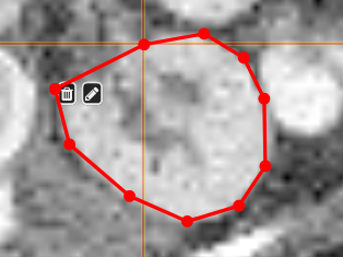
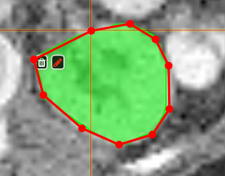
PolygontoolUse the polygon tool to determine a ROI by its outline. You can either create the outline by holding the mouse button down, or click by click. You can also move points of the outline manually after creation. Use trashcan to delete outline, use the pencil to render the polygon into the current ROI enabled for drawing.
|


 move the mouse left/right to adapt size
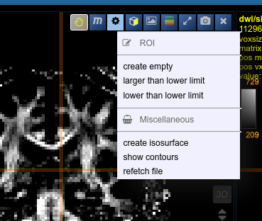
Creating a ROI
To create you always have to give a reference on which basis the underlying geometry the ROI is created. There are several ways to do this:
- Take an existing onto ROI-tool by dragging the hand-icon

from the viewbar of the image (or the file from patienttable) and decide on the type of creation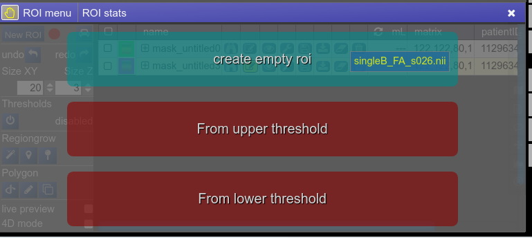
The threshold for creation is the lower limit of the current windowing of the contrast - Or use the cog-wheel item of the viewbar to do the same thing.

- Or just use the "New ROI" button in ROI-tool itself.


 ROI operations
- Morphological Operations: NORA provides the typical 4 operations (erosion, dilation, opening and closing) using a 6-neighborhood in the slicing of the ROI matrix, i.e. the size of the neighborhood varies depending on the underlying matrix size.
- Set Operations: NORA provides intersection, union and set difference. Select
- Remove Salt: Does a connected component analysis and removes components than the given threshold.
ROI statistics
Open the ROIstats window by clicking on the menubar in the ROI-tool
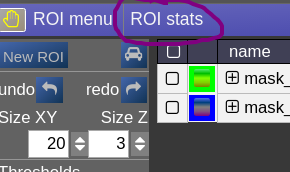
The ROI statitics table appears which computes for all possible combinations of contrasts and ROIs currently present in the viewer the following statistics:
- median of contrast (percentile 50%)
- iqr1/iqr2 - inter quartile ranges (percentile 25% and 75%)
- mean/std - mean and standrad deviation
- volume (in mL)
- area (in cm2, makes only sense when ROI is 2D, or a single slice in the matrix)

Fiber Viewer
NORA includes fiberviewer based on webGL and Babylon.js. The main features are:
- Supports TCK (mrtrix) and TRK (TrackVis) formats
- Fiber Manipulations
- Interactive selection by variable sized spheres
- Interactive deletion by variable sized sphere
- Selection and Deletion of tracts by ROIs
- Selection by sphere sets, (annotation type: poinset)
- Selection by waypoints (annotation type: freeline)
- Selection by DBS electrodes
- Rendering
- Vistmaps (fiber densities)
- Terminalmaps
- LIveupdate of visit/terminal maps
- Tracking
- a simplistic fibertracking algorithm based on tensor/orientationl fields is provided
Starting the fiber viewer
Choose an appropriate background image (like a T1w) and simply drop a tck or trk file into a viewport and the viewer will automatically switch to 3D mode a displays the fibers. An additional viewbar appears, which is associated with the loaded tracts. The viewbars allows you manipulate the streamlines, select subsets, etc. Here a short overview:
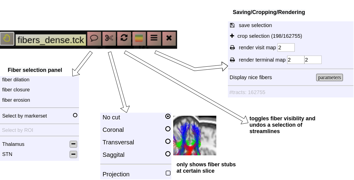
Fiber Selection
- Manually:
Hold Shift key pressed, a yellow sphere appears when hovering with mouse over the tracking, click to select all fibers going through the - By ROI:
- By Annotation:
Cropping Selections and iterative selections.
Some slides explaining NORA' s fiber viewer
Projects and Subject/Studies
Projects
NORA's subject pools are called "Projects". Each user has rights to see a certain subset of projects. The subject/study table on NORA's desktop shows only the subjects/studies of the current project. Projects can differ in their nameing conventions (anonym) and way of storing the data in the backend. They can also have custom processing functions and autoexecution queues.
Subjects/Studies

Filterbars
Use the filter bars to select a subset of studies/subjects. All bars share the following funtionalities: multiple queries are separated by spaces and are interpreted as a "OR" concatenation. If you want to combine expressions that have to be simultanously fulfilled use an explicit "&" sign. All expression have implicity a wildcard at the end of the pattern. For example, search for all patients, whose given name start with A or B, write "A B" into the filter bar of the name column. The "file search" bar can be used to select studies that contain files which match the given file pattern. Explicit wildcards are * and _, where * represents zero or more arbitrary characters and _ represents exactly one abitrary character.
Examples for file searches:
- All studies that have a T1 from a trio:
t1_trio*/s0*.nii - Sometimes naming conventions are different, so use multiple queries:
t1_trio*/s0*.nii MPR_t1*/s*.nii - If you want to restrict for those which have specific study tag:
t1_tri*/s0*.nii & STAG:control
There are special search attributes:
STAG, PTAG, FTAG, JOB, SDESC
For example, search for all studies, which have the tag "control"
STAG:control
Jobs can be queues (q) or running (r) or errornous (e). Find all subjects that have an errornous job
JOB:e
Using Tags
Subjects, studies and files can be decorated with tags. Use the context menu to assign tags. Tags help to group and label items. Files can have special tags
Autoloaders
Marker-Tool
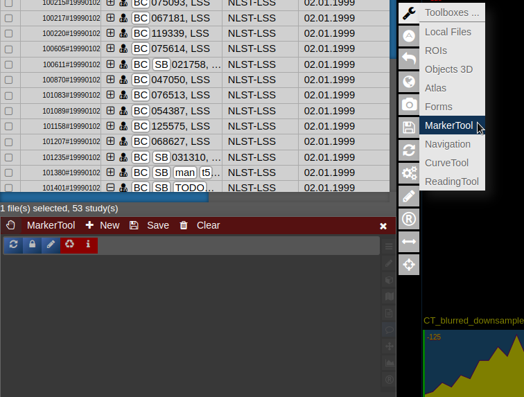
The Marker-Tool enables other types of labels, for instance point-labels.
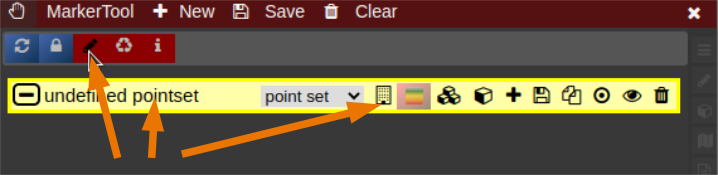
- To open it click on the wrench symbol an select "Marker Tool".
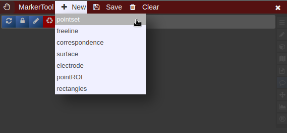
- To create a new pointset go to the menu of the Marker-Tool and select "new+" -> "pointset".
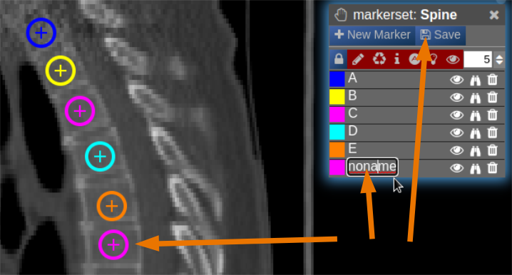
- The pointset can be renamed by clicking on the text in the yellow bar. To enable a list view closer to the image, select the respective list symbol from the yellow bar. To enable adding points by clicking on the image, select the pen symbol.
- Now points are added by clicking on the image. The points are renamed by selecting the text in the list. When finished the pointset must be saved by clicking on the "Save" button. The pointset is stored in a subfolder "annotations" of the current patient.
 |
|
 |
Navigation Tool (alignment and deformations)
NORA provides the possibility to manually align volumetric images (nifits) in a rigid (affine) and deformable fashion. You can interactively translate/rotate/scale the images by holding the Ctrl-key and using the mouse with the yellow crosshair symbol. The deformable transformation is specified by either a set of displacements, or by two set of matching keypoints.
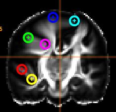
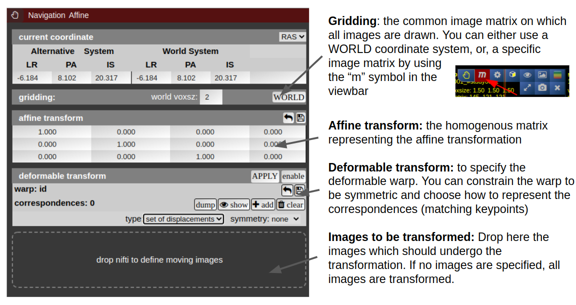
By default, all images are transformed/moving. You can also specify the "moving" images by dropping the nifti into the navigation tool. The moving images are shown in the lower box of the tool. Using the APPLY button(s) the current transformation is applied and written to the niftis defined as 'moving'.
Transformation results are only displayed when the "gridding" is defined to be on one common image matrix. Use either the "world"-image matrix by clicking on the WORLD button or use the "m" symbol on the viewbar of a specific nifti to use the image matrix of this specific nifti. The "world"-system uses a matrix with bounding box including all visible niftis and the voxel size given.
Deformable transformations (warping)
To create a warp field, press the "enable" button in the deformable transform section. By default you can add displacement markers ("correspondences") by pressing the "add" button. The size of the marker defines the extent of the displacement. You can combine multiple displacements. Each displacement is represented by a Gaussian shaped displacement field. By pressing the "dump" button, the displacements markers are rendered as a combined displacement field and markers are deleted. On top of this "dumped" displacement field you can now add again new displacements. Instead of using displacements, one can use two sets of keypoints. Therefore, choose in the "type" combo-box "pair of sets".
URL Calls and Sharedlinks
Shared links (hanging protocols)
Suppose you have arranged a case in the viewer and want to send it to partner, you can save the state and generate a link to access the state via
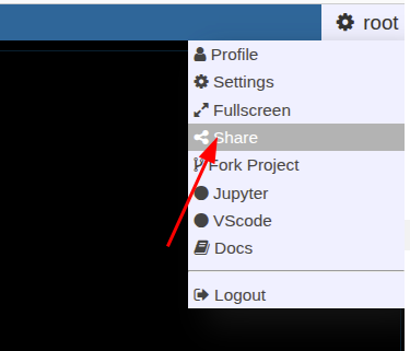
If you have called a link, you can modify and use again the "share" button to overwrite the old link (or create a new one).
URL calls
Suppose you have a NORA project with configured autoloader and want to call a specific case from an external application. You can call NORA via
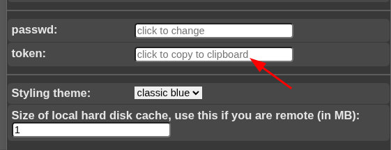
https://nora.ukl.uni-freiburg.de/godzilla/index.php?asuser=root&project=WHATEVER&call={"pid":"yourpatientid","sid":"your studyid","selmode":"yourmode","preset":"youpresetname","user":"username","token":"yourtoken"}The only mandatory options are "user" and "token" for authentication (if you are not already authenticated). Get the token from your profile. Note that you need to create your own password (LDAP authentication is not possible).
Reading Tool
Overview
The Reading Tool enables structured and controlled reading sessions for medical imaging studies. It is designed for both individual and multi-reader scenarios — supporting reproducible reading performance measurements, rater comparison, and annotation-based tasks.
Readings can be configured flexibly: randomized, blinded, repeated, or staged, depending on the study design. Results are stored securely and can be reviewed or exported by reading administrators.
Use Cases
-
Controlled Reading Studies: Measure inter- and intra-rater performance, reproducibility, or the impact of AI assistance.
-
Annotation Tasks: When a single reader annotates or tags cases manually, using the patient table and tag system may be more practical.
-
Training Scenarios: Allow readers to familiarize themselves with representative cases before entering a serious reading phase
Key Features
1. Forms & Rating
-
Create rating forms or questionnaires using the form designer.
-
Readers fill out these forms during reading sessions.
-
Form items can optionally be linked to tags in the patient or study table.
2. Image Interaction
-
Draw annotations, points, or ROIs directly on the images.
-
Combine with predefined autoloaders to automatically load the correct images and view settings.
3. Reading Modes
-
Individual Mode: Each rater works independently.
-
Joint Mode: Multiple raters collaborate on the same session.
-
Blind Modes: Control what metadata or previous results are visible to the reader.
4. Randomization & Repetition
-
Readings can be randomized per patient, study, or image.
-
Repetitions are supported to evaluate reproducibility.
-
Randomization can be deterministic or fully random.
-
Staged Readings: Different stages can present varying image contexts (e.g., raw vs. AI-assisted).
5. Training vs. Serious Mode
-
Training Mode: Assign selected cases for practice.
-
Serious Mode: Conduct the actual study under controlled conditions.
6. Workflow Control
-
Access to the patient table can be restricted or detached for fully controlled sessions.
-
Timing of each reading is automatically tracked.
-
Optionally include reading instructions or external links (e.g., Google Slides presentations).
Data & Results
-
All form entries, annotations, and timing data are stored in the NORA database.
-
Reading results can be reviewed and exported as CSV files by the reading administrator.
Usage of Reading Tool
Open the reading tool (R) in vertical toolbar 
A list of all readings you have permission to access will appear.
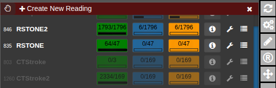
The current progress for each reading is displayed as a numerical indicator showing how many cases have been completed out of the total. To start or continue a reading, click the corresponding button. If available, the Info button opens the reading instructions provided for that session. The Wrench button allows editing of the reading configuration, while the List button displays the collected reading results. To check for newly assigned readings or updates, click Refresh from Server to synchronize with the latest data.
Configure a reading
Click Create New Reading or the Wrench button to edit an existing one. The Form Designer will appear.
general tab
In the general tab, basic settings can be set.
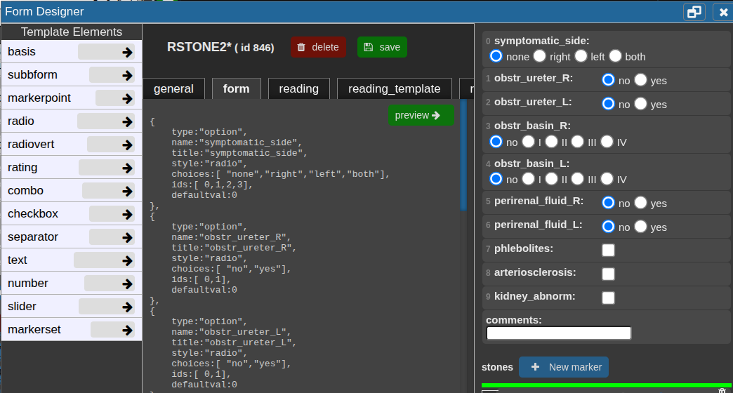
form tab
In the Form tab, define the reading form using JSON code.
Click a template element on the left to copy its JSON snippet, then paste it with Ctrl+V or click the arrow to insert it directly at the cursor position.
Use Preview → to check the JSON and view the rendered form on the right.
Add the property "useastag": 1 to radio or checkbox elements if you want them to act as tags in the patient table.
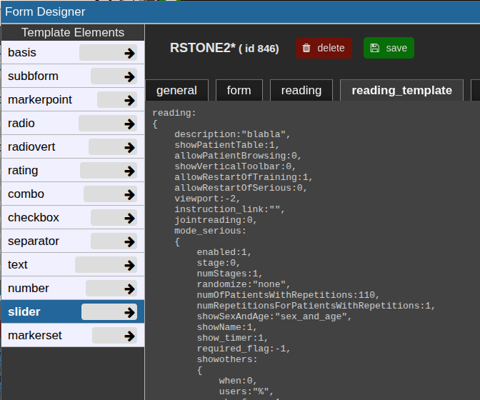
reading tab
This json contain the reading configuration. It consist of several major variables: reading, tools, and viewer.
Most properties are self-explanatory; additional details for specific options are provided below.
For a new reading, it may be empty. If so, go to the reading_template tab and copy the relevant code to start.
The reading_template contains a template for a basic reading. The viewer property always contains the current viewer settings including the autoloaders.
So if you want to change the autoloader / viewer settings, you can modify your current view accordingly, go to reading_template, at copy only the viewer portion or the relevant parts of it.
Training and serious mode
The properties mode_serious and mode_training define the respective configurations for these two stages.
Typically, training cases are marked with a study tag such as "training" and selected using an SQL condition like:SQLCondition: "STAG LIKE '%Training%'".
This allows readers to practice on predefined cases before proceeding to the serious reading phase.
Randomization
By default, readings follow the order defined in viewer.sortOrder and viewer.sortDirection.
To enable randomization, adjust the random property with one of these options:
Testing, debugging and restart
Important Notes
After the test, review the results table to verify that data is stored and displayed correctly.
Before starting the official reading and involving other readers, it is strongly recommended to consult with the system administrators to confirm that the setup is correct and stable, avoiding wasted time and effort.
Data import
PACS Querier
Starting the PACS Query Tool
To start the PACS query tool click on the wrench symbol in the upper left corner. Then click on PACS Query.
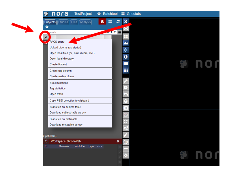
Overview of the Query Tool GUI
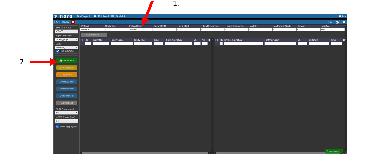
In this window users can search for patients in the pacs.
1. Enter the data of the patient, the patient ID tag can be left empty, in the study date there must at least be a star if the right date is not known. For the PatientName it is important that the lastname is seperated by a ^ from the first name. Depending on your PACS system it might be necessary to always use the full name and appreviations are not accepted.
2. Start the search by hitting the Enter key or clicking on Run Search in the left menu.
Patient Search in the Query Tool
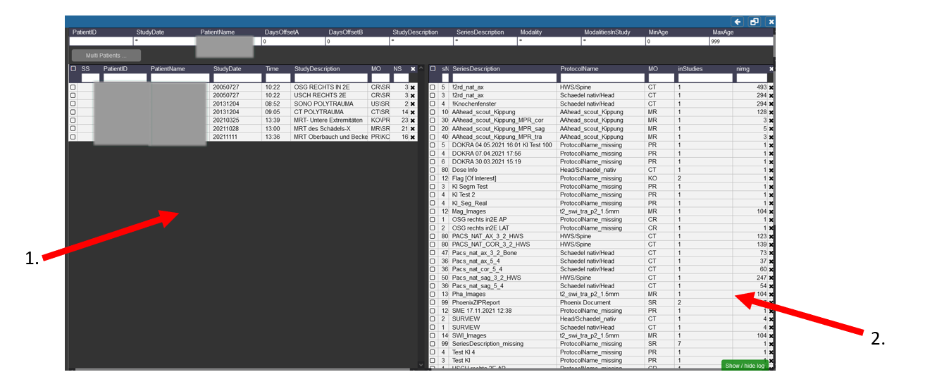
1. On the left side you can see the different Patients with the Names, etc you searched for and the different visits/examinations
That were done for them.
2. Here the different procedures and sequences are listed that you can import into Nora. If the Sequence was acquired for more than one patient or examination there
Is then a number higher than 1 in the Tab inStudies.
Highlighing of Examinations for a Patient
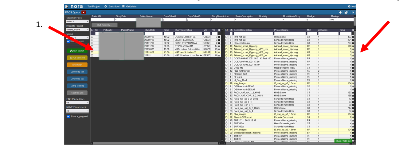
1. To highlight which examinations belong to which patient click on the patient in the left table.
2. Then the examinations which were made during the selected visit of the patient are marked in the right table.
Selection of the patients
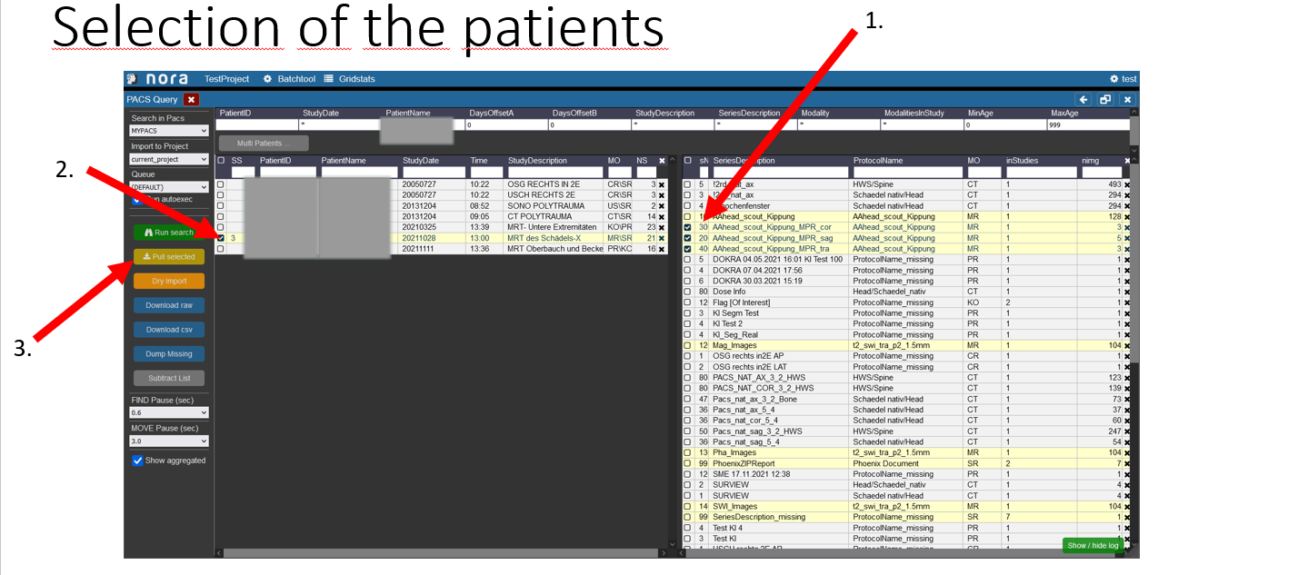
1. First select the examinations you want to import by clicking on the box on the left.
2. In the left table the amount of examinations you selected on the right is showing to which patient they belong, you now have to select the patient by checking the box.
3. To start the import into nora click on the button „pull selected“.
View of the imported Data
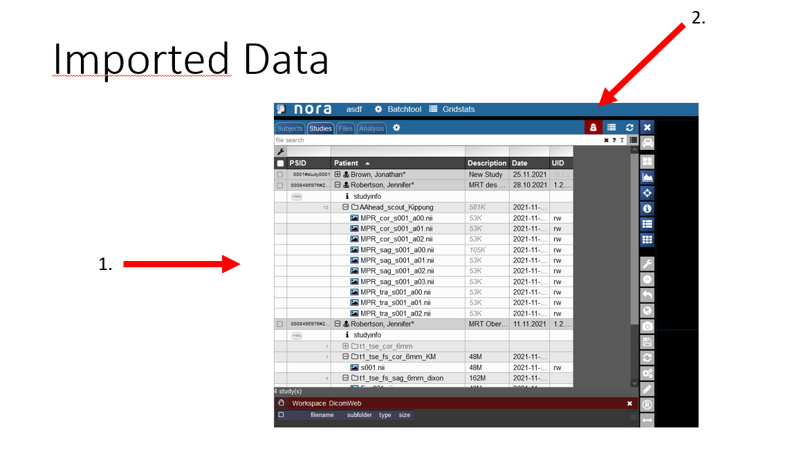
1. Now you can see you imported patient with his examinations.
2. If you click on the symbol the pseudonomyization is deactivated and the real name of the patient is shown. So do not wonder If the name that is initially displate is not the right name.
Manual import
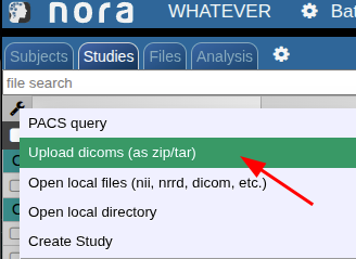
Upload as dicoms
Compress your dicoms into a zip-archive and upload the zip to NORA from here:
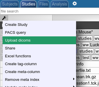
The dicoms are converted with the project specific policies to NIFTIs and imported into the project according to the meta data contained in the data (patient ID, study ID etc.). The import happens on NORA's computing servers.
Import from the server backend (from BASH console) is equivalently possible via
nora -p y YOUR_TARGET_PROJECT --import location_of_folder_or_zip
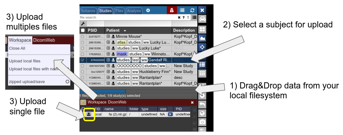
Upload NIFTIs etc.
Any file which is accepted by the viewer and registered by NORA as a proper file can be uploaded into a selected subject. Use drag&drop from your local filesystem to NORA's desktop (1), then select a subject/study as target for upload and upload the data (2). The, just use the menu or the upload buttons to upload the files (3). You can also decide for zipped upload. If the dropped data also contain meta information (like DICOMs are Bruker imaging data), you can also use this information during upload for the subject/study assignment: just use "Upload local files with native PID" for uploading the files. If the corresponding subject is not existing in the project, the study is automatically created.
Create Project From Existing Data
Dicom import via HTTP POST
You can upload dicoms from command line via a REST API. For example, use wget/curl (linux) or iwr (Windows). Here is example using curl
curl "https://nora.ukl.uni-freiburg.de/godzilla/index.php?project=WHATEVER"\
        -F 'call={"cmd":"import","user":"donaldduck","token":"@CRYPT@yourtoken"}'\
        -F 'thefile=@/a/path/to/a/zipped/dicomfolder/data.zip;type=application/zip'
The data is uploaded and a job on the cluster is started for conversion to nifti.
It's equivalent to using the web interface (Upload dicoms)
Processing
General
The batchtool was created out of the needs to apply common neuroimaging pipelines (like SPM, FSL, Freesurfer) on medium sized projects (10-1000 subjects) in a convenient and efficient manner. One of the major objective of NORA's batchtool is to deal with heterogenous data. Typically, files (a.k.a. image series, or any other filecontent) are selected by file patterns, which can iteratively generalized. Errors can be easily tracked by a simple error logging system. For example, it is simple to select a errornous subgroup and rerun a modified job for them, which was corrected for the error. Processing pipelines (batches) are a simple linear series of jobs. Depending on the relationship between individual jobs, they can run serially or in parallel.
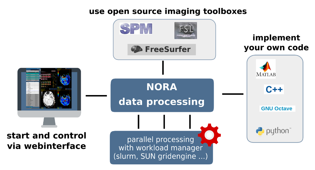
Figure 1: Design principle
In conclusion, what it provides:
- Convenient selection of subject/study sets to apply certain processing pipelines
- Definitions of inputs via Tags or filepatterns with wildcards
- Composition of processing pipelines based on predefined scripts/jobs (mostly MATLAB), or custom MATLAB/BASH/Python code
- Submission of jobs to a cluster (Slurm/SGE) with direct access to logs and errors
Batchtool
The Batchtool Window
Consider Figure 2 below: the subject/studies table on the left is used for the selection of subject/studies on which you want to run your batch. You can use the filter bars to create the subgroup you want to work on (see Subject/Studies table). Select "Batchtool" on the top toolbar (A) to open the batchtool. Figure 2 shows the structure of the Bacthtool window. It allows to compose the batch out of single jobs. Jobs are added from the menu (D). You can save batches (E), which then appear in the batch list (C). To open an overview of currently running jobs open the "Gridstats" window (B) or (H).
Batches are launched for every subjects/study independently in parallel. The jobs within a batch run sequentially. You can also choose different running option (see (G) in Figure 2). Depending on the selection level (subjects or studies), the batches are iterated over subjects or patients
![]()
Imagine a scenario where you have multiple studies per patient, which have to be linked in some sense. Then, the subject level is appropriate. For example, think of a neuroimaging analysis where you a have a CT study (which contains, e.g. electrode information) and a MR study (which contains soft tissue anatomical information), or think of a simple longitudinal analysis. Otherwise, if your your studies should all be treated in an equal manner, the study level is appropriate.
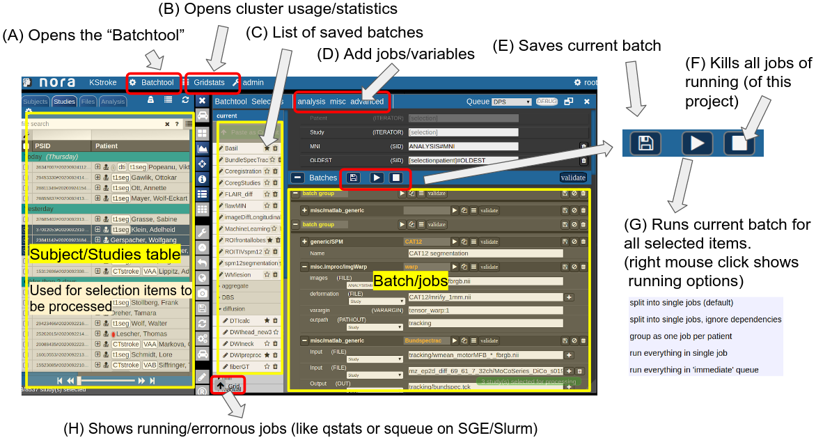 Figure 2: Batchtool overview.

The Anatomy of a Job
A job consists of a list of arguments. There are several types of arguments:
-
FILE
All input images/series (or any other type of files) are given as FILE arguments. Usually you give a file pattern instead of an explicit filename. A fIle pattern is a combination of subfolders, filename and wildcards. For example: t1*/s0__.nii. I refers to all files contained in a folder starting with t1 and whose filename matches "s0___.nii" . The asterisks (*) is a placeholder for an arbitrary character sequence, an underscore "_" for a single character. Internally, the wildcards are the same as for SQL "like" statement (the '*' is replaced by '%'). A FILE argument also includes a reference to a study or patient. Depending on the selection level (subject or study), different "study references" are possible. See below for more about "study references". -
OUT
A name of a file including the subfolder. No wildcards are allowed here. Depending on the selection level there are again different study references possible. A output file may be tagged by putting in the OUT field "myoutputfilename TAG(mytagname)". -
PATHOUT
Same as OUT but refers to foldername instead of a filename. - NUMERIC
- STRING
- LOGICAL
- OPTION
Study References and study selectors
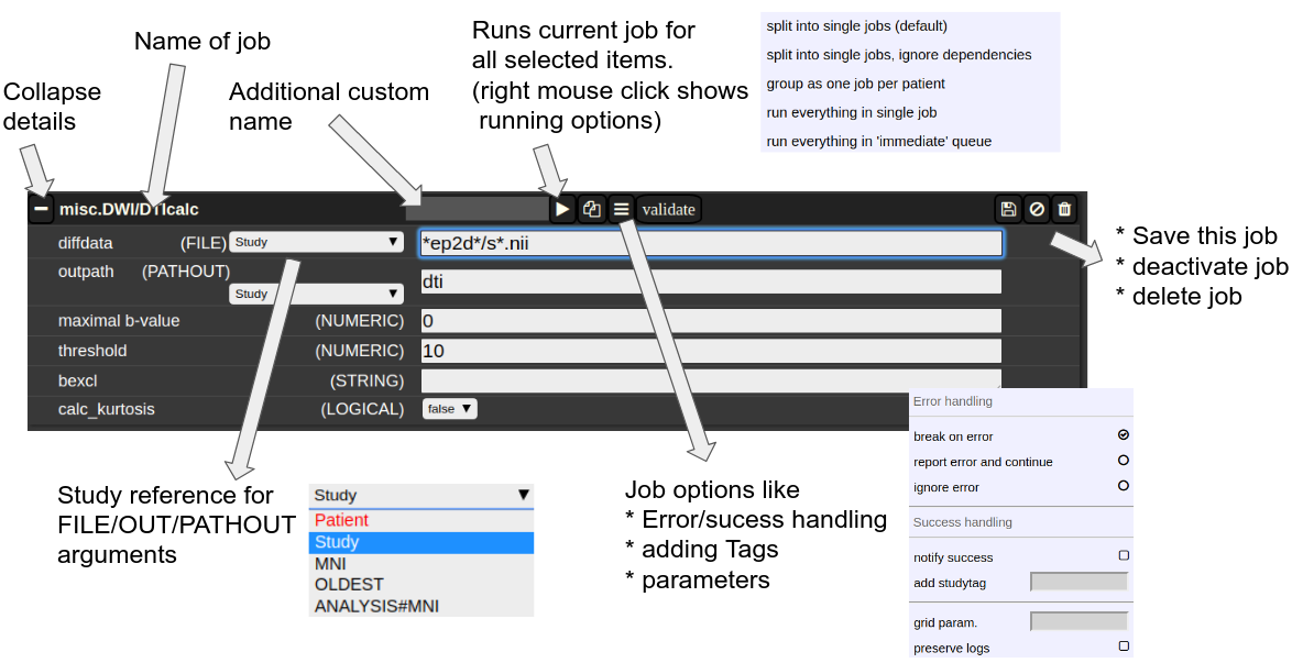
Figure 3: The anatomy of a single job.
Cluster Managment/Monitor (Gridstats)
To monitor the integrated cluster environment there is a simple table based overview, which provides accessto job logs and job modifications. One can also sort and search the current job statistics to selectively monitor or kill/suspend jobs. While finished jobs just disappear by default (you can change this in the settings), jobs that have produced an error are kept for further analysis. Note that the job information is also available on subject/study level (see Figure 2) as small indicators. To get further information about the job, you can click on the function cell and a JSON-representation of the job is displayed. A click on the subject cell selects the corresponding subject/study in the table.
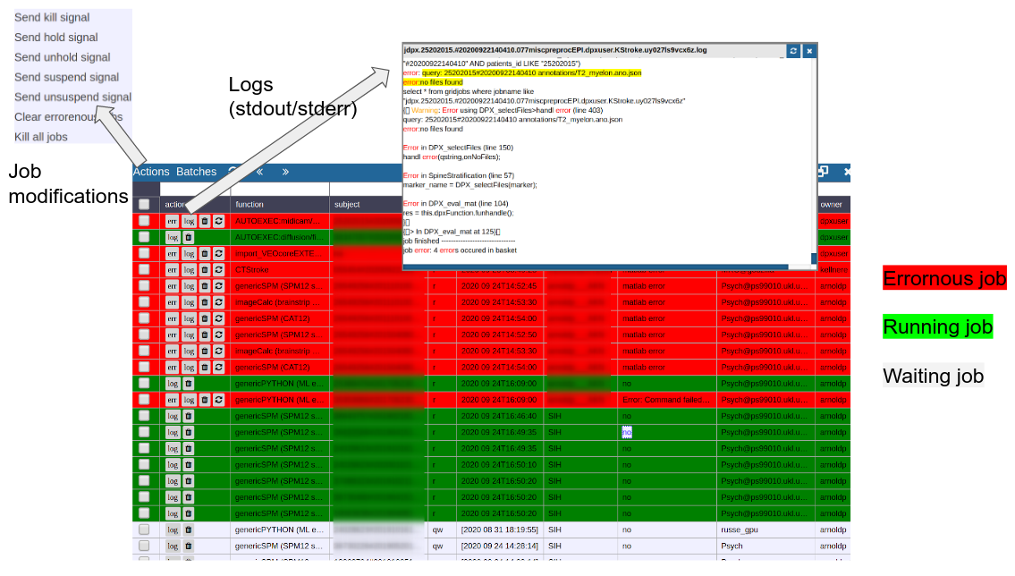
Figure 4: Gridstats: monitoring and control of the cluster environment/resource managment (Slurm/SGE)
Jobs
Generic jobs
There are a multitude of predefined algorithms (mostly MATLAB) in NORA; however you can also implement your own scripts directly by using generic jobs. Currently there are three types of languages possible:
- BASH
- Python
- MATLAB
A generic jobs basically provides a field where you can enter simple expression or a full script in BASH/Python or MATLAB. Arguments from NORA are passed to the script by simple variable naming conventions.
For BASH/Python scripts input files (and all other parameters) are referenced by variables with a $-prefix with a special naming convention. For example, file arguments are referenced by $f1-$f9. Once NORA finds such an expression it automatically adds a corresponding row at the bottom of the job, which can be filled by the appropriate file patterns. The same holds of output arguments (represented by $o1-$o9) and output paths (prefix 'p'). Other parameters (STRING,NUMERIC) are referenced by prefixes 's' and 'n'.
In MATLAB the approach is a little bit different. You can manually add input/output arguments by using the "plus" sign and refer to the arguments by ordinary MATLAB variables. As input you have a series of cell-Arrays (input1, ..., inputN), as output a series of strings (output1, ..., outputN).
The input and output filenames are resolved to absolute paths that may be used directly.
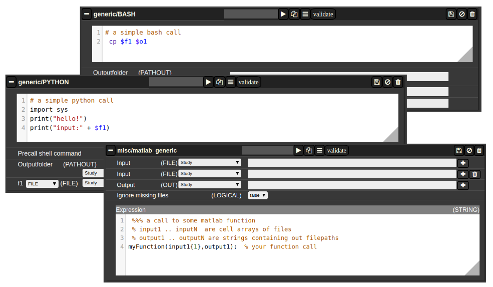
Figure 4: Generic Jobs
The Nora backend and related software is available to the jobs. The backend command is named nora. This allows bash jobs like: nora -a $1 --addtag mytagname. This example adds a tag to a file that was selected for processing, by making use of the backend.
Jupyter Notebooks
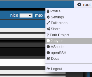
Nora allows to submit cluster jobs which launch jupyter lab. There are several ways:
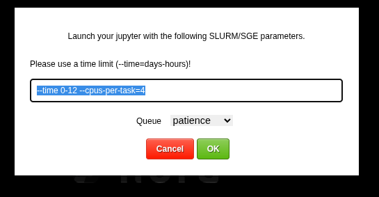
- Go to your right upper corner, and choose jupyter

This allows you to launch a jupyter lab on the cluster. You can choose slurm parameters for the job

The root folder of the notebook will be located on you persistent home folder on the cluster. - For debugging the batchtool can open a job in a jupyter notebook:

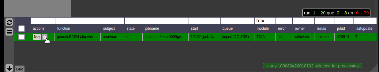
The jupyter notebook is opened in a new browser-tab (make sure your browser allows pop-ups for Nora):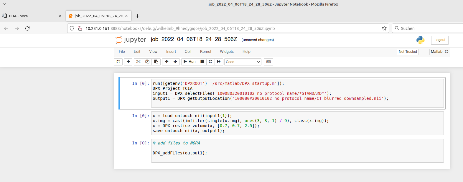
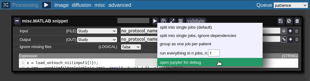

When finished with debugging close the tab. Don't forget to kill the jupyter-notebook job in the grid view. The view may be opened on the bottom of the batch tool.
Fibertracking, Streamline Analysis
Some slide explaining NORA's fiber viewer
Streamline Analysis
thanks to Andrea dressing for the tutorial
Segmentation (Deep Learning)
Training and Using Segmentation Models
The Batchtool allows you to train custom 3D segmentation models on your own data and apply them to new studies.
Here's a short tutorial on how to use the patchwork segmentation model (Deep Neural Patchworks: Coping with Large Segmentation Tasks, Reisert et. al, 2022)
1. Training a Segmentation Model on Your Data
In the Batchtool:
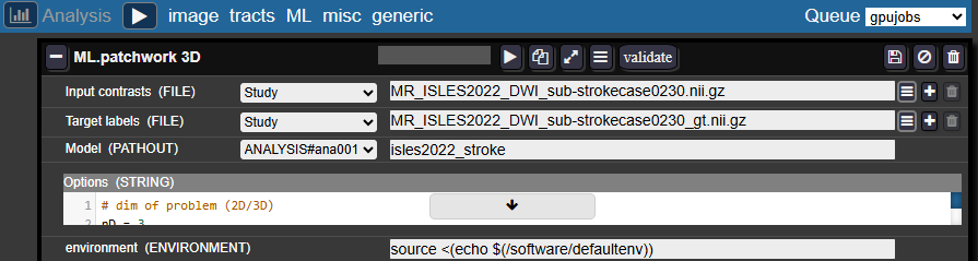
- Create a new Analysis → ML → Patchwork 3D
Entry fields:
- Inputs contrasts and Target labels: Enter the filenames of your images and masks as they appear in each study
- Model: Select an analysis folder (create one in your project if needed) and provide a name for your model folder, for example:
isles2022_stroke
Configuration:
- In the Studies panel, check the studies you want to train the model on
- Select a job queue and run the analysis
- The job should appear in the Gridstats. You can monitor training progress in the log.
Training notes:
- The default number of iterations is 2500
- The model is saved after each epoch, so you can also terminate the job early if performance is satisfactory
2. Applying the Trained Model to New Studies
In the Batchtool:
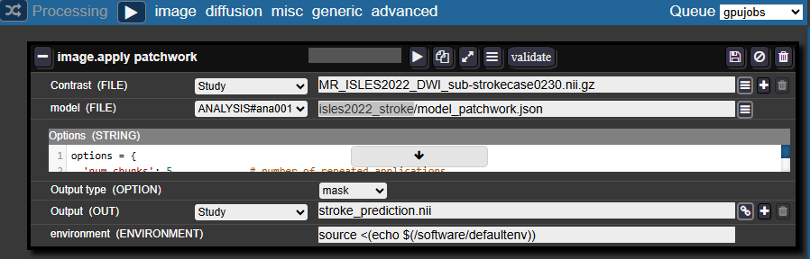
- Create a new Processing → Image → Apply Patchwork
Entry fields:
- Contrast: The filename of your image in your studies
- Model: Select the same analysis folder and specify:
<model_folder_name>/model_patchwork.json- For example:
isles2022_stroke/model_patchwork.json
- For example:
- Output type: Select Mask
- Output: Specify the desired name for the resulting mask
Configuration:
- In the Studies panel, check the studies you want to apply the model to
- Select a job queue and run the processing
- Monitor the job progress through the logs in Gridstats
Detailed documentation :
Installation
NORA inside a Docker
Install Docker on your host system
First, install docker, git and jq on your host system
sudo apt-get install docker.io git jq
There might be an issue with the DNS address in docker. To check this, run
docker run busybox nslookup google.com
If the host cannot be reached, grep the address of your DNS server
nmcli dev show | grep 'IP4.DNS'
create the file /etc/docker/daemon.json and insert the address as
{
"dns": ["yourDNSip", "8.8.8.8"]
}
then restart docker
sudo service docker restart
go back to the busybox above and check if it works now.
Now, you should add your user to the docker group, otherwise you have not to sudo all NORA commands
sudo adduser <username> docker
!!! you have to re-login to make these changes apply !!!!!!
Clone the git repository
NORA was historically named DPX. Note that this name might still often be used in the following. Clone the repository into to a temp folder, or to your favorite program place.
Let's say we clone to your home directory into ~/nora
git clone https://<yourname>@bitbucket.org/reisert/dpx.git ~/nora
If want to use NORA in a multi-user environment you might want to create a specific group (we usually use dpxuser) and change the group of that directory (recursivey) accordingly. In any case, you have to set the s -flag and some ACLs recursively to that dir (you might have to run this as sudo. In this case make sure to apply it to the correct ~/nora directory !! )
find ~/nora -type d -exec chmod g+s {} +
If want to manage rights by ar group user
chgrp -R NORA ~/nora # if you manage your right via usergroup NORA./dp
nonetheless
setfacl -R -d -m g::rwx ~/nora
Initial configuration
Go into the nora directory and run ./install
This will create some local config files in the "conf" directory (for details see separate section below).
NORA has 3 modules
- Frontend: webserver with image viewer
- DICOM node to receive images from a PACS
- Backend: processing module (depending on your preferences matlab or nodejs and slurm or SGE based)
By default, all three modules are enabled. To run NORA in this default configuration edit main.conf and set at least MATLABPATH: <your-path-to-matlab>
If you are behind a proxy, it might also be necessary to set the proxy (maybe even with user/password)
DOCKER_http_proxy:" ... "
Also set the user Nora should act as in the main.conf
DPXUSER: " ... "
DPXGROUP: " ... "
Build the docker image
Your main function to control NORA is dpxcontrol. You can always run
./dpxcontrol
to get more help. To build the DOCKER image, first run
./dpxcontrol docker build
This will take a while. If everything went well, start all modules with
./dpxcontrol start
If something went wrong during installation / starts, there might be old 'zombie' containers. In this case you will be suggested docker commands to remove them. You can also start with --forceto autoremove old NORA containers.
To check the status, now use
./dpxcontrol status
If at least the first point, Docker, is running nicely, you should be able to log into the Webinterface. (see below)
Log into the Webinterface
Now, open a web-browser and go to localhost:81. Default login is
user: root
password: dpxuser
There are several options to create new users. You can either connect to an existing LDAP server, or just create users based on the internal user management of NORA (see Administration section for details).
Troubleshooting and testing
Most log files are written into
<path-to-nora>/var/syslogs/
These can also be seen from the admin dialog at the top of the webinterface. If the daemon is not starting (or stopping again, red status) check the daemon.log for more info. In case of a license error, maybe you have to forward your MAC adress to Docker (see main.conf for more info)
For other system parts, there are also some test functions
./dpxcontrol test [slurm | email | more_to_be_programmed]
Upgrade the database
When your daemon is running nicely, it might be necessary to upgrade the initial database with
./dpxcontrol matlab updatedb
Autostart on system startup
To automatically start NORA when your computer starts, you can for example add <path-to-nora>/dpxcontrol start --force to your /etc/rc.local
Slurm setup
A proper configuration of slurm is a science on its own. Ask google for more information. If you are running slurm inside docker (default), the conf/slurm.conf is used and you do not have to do too much. Otherwise, if docker is installed outside (this should be the correct practice) you have to it install via
sudo apt-get install slurm-wlm
on a deb-system and set
DOCKER_run_daemon_in_docker: 0,
in the <path-to-nora>/conf/main.conf file. For configuring slurm itself there is a configurator interface via html, which you usually find here
which generates a conf file /etc/slurm-llnl/slurm.conf where you have replace the hostname by the machine you are running NORA on. Further, the partitions have to specified. NORA has as default two partitions
(computing queues) DPXproc and DPXimport, which have to specified in the slurm.conf like in this example:
# COMPUTE NODES
NodeName=hostname CPUs=8 State=UNKNOWN
PartitionName=DPXproc Nodes=hostname Default=YES MaxTime=INFINITE State=UP
PartitionName=DPXimport Nodes=hostname Default=YES MaxTime=INFINITE State=UP
Alternatively, if you have an existing SLURM running with predefined paritions, you can change the paritions (queues) in NORA’s configuration in <path-to-nora>/conf/main.conf (SLURM_QUEUES)
Also consider
./dpxcontrol test slurm
for testing whether your slurm configuration is working.
General Configuration
All configuration files are located in <path-to-nora>/conf directory. The configuration files are
- main.conf - includes all major configurations, responsible for
- Location of external programs (MATLAB etc)
- DOCKER port forwarding
- Daemon beahviour
- Import behavior (dicoms etc)
- Mysql information
- signin/signup behaviour, LDAP configuration
- Backup behavior
- pacs.conf - includes all information how to connect to external dicom nodes
- routes.conf - ip-addresses of DB, and routes of mount dirs (depending on hostnames diffferent mount locations are possible
- slurm.conf - slurm configuration
- smail.conf - mail configuration
Administration Backend
Command line Interface (BASH)
You need a PATH to <path-to-nora>/src/node
Call
nora
any get help
 NORA - backend
usage: nora [--parameter] [value]
--project (-p) [name]
       all preceding commands refer to this project

MANAGEMENT
--sql (-q) [sqlstatement]  [--csv]
       executes SQL statment and return result as json (or as csv if option is given)
--add (-a) [file] ...
       adds list of files to project
       option: --addtag tag1,tag2,... (tags the files)
--del (-d) [file] ...
       deletes list files
--del_pat (-dp) [patient_id] [patients_id#studies_id] ...
       deletes list of patients/studies
--out (-o) [filepattern]
            computes absolute outputfilepath from filepattern (see description of filepattern below)
--pathout (-pa) [filepattern]
            computes absolute outfilepath from filepattern
--select (-s) [--json (-j)] [--byfilename] [filepattern]
            returns files matching filepattern, if --json is given, files are return as json filepattern
            if --byfilename (together with --json) is given, files are restructered by filename
--addtag tag1,tag2,... -s [filepattern]
            add tag to file
--rmtag tag1,tag2,... -s [filepattern]
            removes tags fromfile
--launch (-l) [json]
            launches batch from json description
--createproject (-c) [name] [module]
            creates a project with [name] from [module] definition
--admin [parameter1] [parameter2] ...
            calls the admin tools (see nora --admin for more help)

PROCESSING
--launch json
            launches a NORA job given by json
            options: --throwerror
                     --handle_job_result (emits DONE signal, when ready)
--launchfile jsonfile
            same as --launch but json given by fileref
--launch_autoexec psid
       launches the autoexecution pipeline of the project for the patient specified by psid
--import srcpath
            imports dicoms located in sourcepath to given project
            options: --autoexec_queue (if given autoexecuter is initiated, use DEFAULT to select default autoexecution queue given in config)
                     --handle_job_result (emits DONE signal, when ready)
                     --extrafiles_filter: if there are non-dicom files in your dicomfolder and you
                    want to add them to your patient folder, then, give here a comma-separated list of
                    accepted extensions (e.g. nii,hdr,img)
                     --patients_id PIZ (overwrite patients_id of imported data with PIZ )
                     --studies_id SID (overwrite studies_id of imported data with SID )
                     --pattern REGEX (use REGEX applied on srcpath of dicoms to overwrite
                                patients_id/studies_id, example:
                          --pattern "(?<studies_id>[\w\-]+)\/(?<patients_id>\w+)$"

OTHER
--exportmeta [filepattern]
            exports meta data as csv. Meta content from files matching [filepattern] are exported
            options: --keys a comma separated list of key-sequences, which are exported [optional]
                   a key sequence is given by a dot-separated list, where the first key refers to the name of
                   the json-file (as multiple jsons might be contained in the query). A wildcard * is possible
                   select multiple keys at once
                     examples:
                   nora -p XYZ --exportmeta '*' 'nodeinfo.json'       // gathers also patient info
                   nora -p XYZ --exportmeta '*' 'META/radio*.json' --keys '*.mask.volume,*.mask.diameter'
MATLAB Interface
To setup NORA for MATLAB you change to the folder
<path-to-nora>/src/matlab
at the MATLAB prompt and start DPX_startup. This sets up all necessary paths and the database connection. To test the DB connection, make a call to DPX_Project. This should list all created projects (initially only the default project). There are a variety of management commands to manage users/project/data etc. Here a list of important ones:
- General
- DPX_startup - sets up NORA
- DPX_Project - choose a project
- DPX_getCurrentProject - get the current project information
- DPX_SQL_createUser - create a user
- DPX_SQL_createProject - create a project
- File selection
- DPX_getOutputLocation - compute the path to certain output
- DPX_selectFiles - select files based on pattern
- DPX_getFileinfo - get additional file information (no database involved)
- DPX_SQL_getFileInfo - get information from database for this file
- Processing
- DPX_demon - start the processing deamon
- DPX_debug_job - execute a debug job at the MATLAB command prompt
DPX_SQL_clearGridCmds - clear all jobs from the pipeline
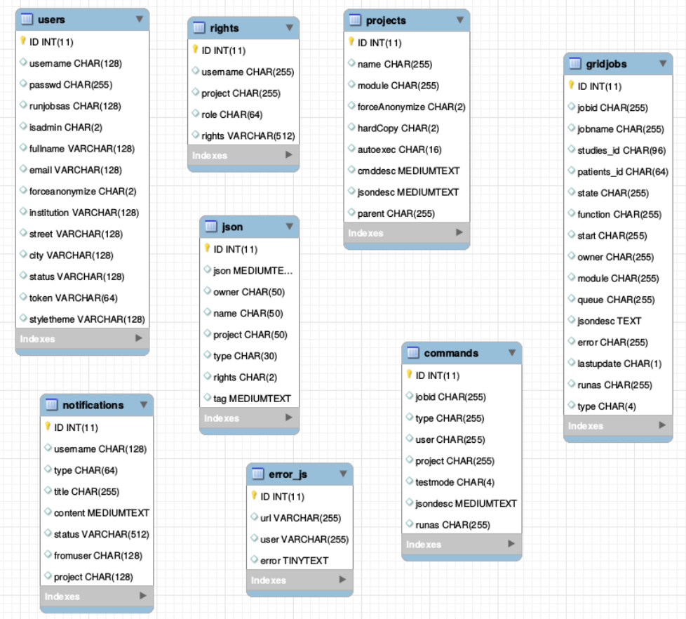
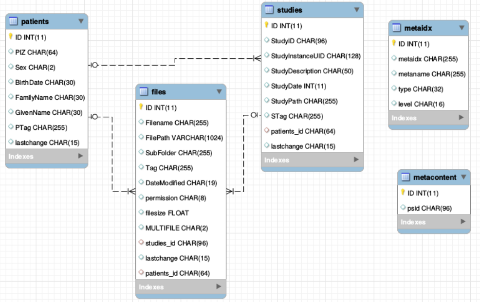
The Database
There is one general database scheme containing information about users, projects, jobs, settings etc.
You can see below the table schemes.
- Projects/User management
- projects
- users
- rights - who can read which project in which role
- Batch/Jobs
- gridjobs - contains submitted and running jobs (mirror of qstat or squeue)
- Commands - contains jobs submitted from web interface, but not yet submitted to resource management system.
- Miscellaneous
- json - various types of jsons (saved batches, shares, settings, states etc.)
- notifications
- error_js
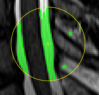
Segmentation Assistant for ROItool (nnInteractive)
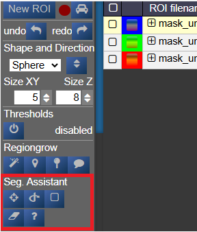
This assistant allows users to create and refine 3D ROIs using interactions. Images, masks, and successive interactions are processed by a deep learning model hosted on a remote server.
The current version of the model is nnInteractive (Isensee, Rokuss, Krämer et. al., 2025). nnInteractive repository
1. Usage
First, select an ROI from the ROI list to make it the active target for segmentation.
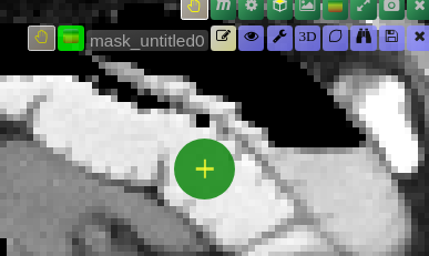
Point Interaction
- Click the Point icon (crosshairs) to activate Point mode
- Left-click on the image to add a positive point (to include an area)
- Right-click on the image to add a negative point (to exclude an area)
- The segmentation will be updated immediately. Click the icon again to deactivate
- To add multiple points before updating the segmentation, hold down the Q key while adding points. Release the Q key to send all accumulated points at once
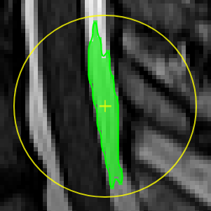
Scribble Interaction
- Click the Scribble icon to activate Scribble mode and draw a scribble on the image
- Click the + button to run a positive interaction (add areas)
- Click the - button to run a negative interaction (remove areas)
- Scribbles are cleared after each interaction, allowing you to add more
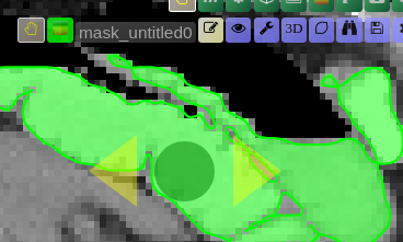
BBox Interaction
- Click the BBox icon (square) to activate Bounding Box mode and draw a box on the image
- Click the + button for a positive interaction (segment inside the box)
- Click the - button for a negative interaction (exclude area in the box)
- The box is cleared after each interaction
Reset Interactions
- When editing the same ROI, all previous interactions are kept in memory server-side to guide the segmentation
- Click the Reset icon (eraser) to erase all previous interactions and start fresh
2. Server Setup
The segmentation server must be running, typically on a machine with a GPU. First, navigate to the src/python/segmentation_assistant_server directory and launch the setup.sh script (requires internet access):
cd src/python/segmentation_assistant_server
./setup.sh
This will create a Python virtual environment and install the necessary dependencies.
Next, start the server from a computing node with:
cd src/python/segmentation_assistant_server
./start.sh
3. Client Configuration
Once the server is running, it will log its port. You must update this client's configuration to point to that address.
Edit the file: conf/segmentationserver.conf
Set the REMOTE_SEGMENTATION_BASE_URL to the server's address, for example:
{"REMOTE_SEGMENTATION_BASE_URL":"http://<SERVER_IP>:PORT"}Important: You must restart Nora for the changes to take effect.